


Executive Summary
The primary bottleneck for running Large Language Model (LLM) agents on local hardware is not just the model size (weights), but the “Memory Wall”—the escalating resource cost of the KV (Key-Value) cache. For sophisticated agents, the memory required to maintain conversation history and context can equal or exceed the memory required for the model itself. For example, a 70-billion parameter model (70B) requires approximately 42 GB of VRAM for its weights at a standard 4-bit quantization, but a full 128,000-token context window can demand an additional 43 GB of memory.
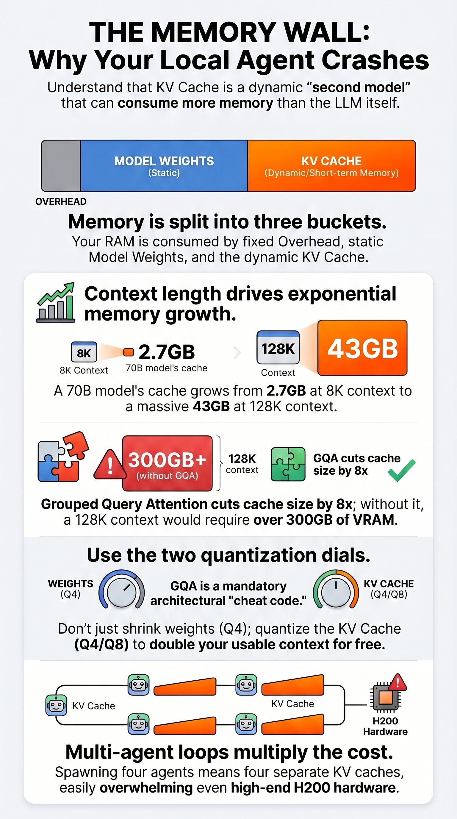
Successful local agent deployment requires balancing three specific memory “buckets”: fixed overhead, model weights, and the KV cache. While weights are static, the KV cache is dynamic, expanding with context length and the number of concurrent requests. To bypass the “Memory Wall,” developers must utilize specific architectural choices like Grouped Query Attention (GQA) and software-level “dials” such as KV cache quantization. This document synthesizes the technical requirements, formulas, and hardware implications for managing these resources in local environments.
--------------------------------------------------------------------------------
The Three-Term Memory Budget
Running a local agent involves a predictable arithmetic of memory allocation. Total memory consumption is divided into three distinct categories:
Bucket
Description
Scale/Cost
1. Fixed Overhead
The baseline cost for the backend (e.g., llama.cpp) to exist.
~0.75 GB (Measured baseline)
2. Model Weights
The static size of the model, determined by parameter count and quantization level.
Fixed (e.g., 70B at Q4 is ~42 GB)
3. KV Cache
The model’s “short-term memory” that stores key and value tensors for every token in context.
Dynamic (Moves with context length and concurrency)
The “Second Model” Phenomenon
In chatbot scenarios, the KV cache is often negligible. However, agents are not chatbots; they carry forward system prompts, tool definitions, full message histories, and retrieved documents, re-reading this data at every step. At high context lengths (128k tokens), the KV cache becomes a “second model” sitting in memory, doubling the total hardware requirement.
--------------------------------------------------------------------------------
The KV Cache: Mechanics and Formulas
The KV cache cost is not mysterious but follows a specific mathematical formula. Understanding this formula allows for precise hardware planning.
The KV Cache Formula
The memory cost of the KV cache is calculated as: Layers × KV Heads × Head Dimension × Context Length × 2 (Key/Value) × Bytes per Element
The Impact of Grouped Query Attention (GQA)
GQA is a critical architectural feature baked into modern models like Llama 3.1. It reduces the number of KV heads relative to query heads.
Example: Llama 3.1 70B uses 8 KV heads instead of 64.
Efficiency Gain: This architecture cuts the memory cache by a factor of eight. Without GQA, a 128k context for a 70B model would require ~320 GB of VRAM, making it impossible for consumer hardware.
--------------------------------------------------------------------------------
Technical Levers: The “Dials” of Optimization
There are two primary “dials” available to shrink the memory footprint of a local agent. Most users only adjust the first, leaving significant efficiency on the table.
Dial 1: Weight Quantization
This involves shrinking the model weights (e.g., using 4-bit quantization or “Q4”). This is the standard “sweet spot” for maintaining quality while reducing the initial memory footprint.
Dial 2: KV Cache Quantization
This is a separate operation from weight quantization, typically toggled via inference flags (e.g., in llama.cpp).
8-bit Cache (Q8_0): Halves the cache size with negligible quality cost.
4-bit Cache (Q4_0): Quarters the cache size. While there is a task-dependent quality impact, it allows massive context windows on mid-tier hardware.
Practical Impact: On a 70B model with 34 GB of free VRAM, full precision holds ~109k tokens. Switching to 8-bit quantization doubles that to ~218k tokens.
--------------------------------------------------------------------------------
Agentic Context Inflation
Agents consume context significantly faster than standard LLM interactions due to their operational overhead.
The Tooling Tax: Tool definitions are extremely “expensive.” A single Model Context Protocol (MCP) style operation can consume 32,000 to 82,000 tokens of context. In contrast, a plain command-line call costs roughly 200 tokens.
Multi-Step Compounding: Because agents re-read their instruction manuals and history at every turn, research and coding agents routinely operate in the 32k to 128k token band.
The Concurrency Trap: The KV cache cost is multiplied by the number of concurrent requests. Running four sub-agents simultaneously at 128k context would require ~160 GB of KV cache alone, exceeding the capacity of even high-end enterprise cards like the H200 (141 GB).
--------------------------------------------------------------------------------
Hardware Implications and Performance Trade-offs
The distinction between “it fits” and “it’s usable” is defined by memory bandwidth and architecture.
Unified Memory vs. Discrete VRAM
The 24GB Limit: Standard discrete cards (e.g., RTX 3090/4090) cannot hold the weights of a 70B model. Spilling into system RAM causes speed to collapse to unusable levels.
Unified Memory Advantage: Platforms like the Mac (M4 Max) or Strix Halo provide large unified memory pools (up to 128 GB), which are essential for holding both the 42 GB of weights and the 43 GB of KV cache required for long-context 70B agents.
Speed vs. Quality
The Bandwidth Ceiling: On low-bandwidth boxes, the time to fill and read the cache increases with context length.
Reasoning Models: Running high-token-output reasoning models on “budget” hardware may result in speeds as low as 10–12 tokens per second if weights are pushed to 8-bit quality. This can turn a single response into a multi-minute wait, making interactive use impractical.
Silicon-Specific Doors: Modern hardware uses tricks like NVFP4 (4-bit format) to move less data per token. However, these are often architecture-specific; for instance, RDNA architecture lacks FP8 hardware, closing certain acceleration paths available to NVIDIA users.
--------------------------------------------------------------------------------
Conclusion: The Final Budget Calculation
To determine if a local machine can truly support an agentic workload, the following calculation must be performed:
Total Memory Needed = Overhead + Weights + (Cache-per-Request × Concurrency)
The “Memory Wall” is hit when the dynamic growth of the third term (Cache) exceeds the remaining VRAM after the first two terms are loaded. Managing the “second model” (the cache) through GQA-equipped models and KV quantization is the only way to enable high-capability agents to function on affordable local hardware.


